Logistic Regression in Machine Learning

Before studying logistic regression, I would recommend you to go through these tutorials.

• Linear Regression in Machine Learning
• Gradient descent vs normal equation

The first and most important thing about logistic regression is that it is not a “Regression” but a “Classification” algorithm. The name itself is somewhat misleading. Regression gives a continuous numeric output but most of the time we need the output in classes (i.e. categorical, discrete). For example, we want to classify emails into “spam” or “not spam”,  classify treatment into “success” or “failure”, classify statement into “right” or “wrong”, classify transactions into “fraudulent” or “non-fraudulent” and so on. These are the examples of logistic regression having a binary output (also called dichotomous). Note that the output may not always be binary but in this article, I merely talk about binary output.

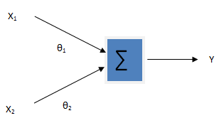
The following block diagram illustrates the logistic regression model

[ Y =  func (theta_0 + theta_1x_1 + theta_2x_2) ]
The first part of figure is same as the linear regression. The output of linear regression is now fed into the function that normalizes the input into the range of [0,1]. Here we need a function that, when given the variable in range   [-∞, +∞], produce the output in the range [0,1]. The sigmoid function (also called logistic function) is the solution for this. The equation of logistic function is given by
[ h_theta(x) = frac 1 {1 +  e^{-theta^Tx}} …………. (i)]
The exponential part i.e. θ^Tx is the output of linear regression.

The simple plot of this function would be

From figure, it is clear that the value of θ^Tx smaller than about -4.6(approx.) gives the value of 0 and value of θ^Tx greater than +4.6(approx.) gives the value of 1. So the logistic function maps any range of values to the range [0,1] and this confirms that h_θ(x) will be between 0 & 1 unlike the linear regression where h_θ(x) can take any values between [-∞, +∞].
For the classification, we need a decision boundary that separates one class from another. The simple linear decision boundary would be

It means we define a threshold that separates the positive class from negative class. For example, in spam classification problem, after feeding the input attributes to the model, if we get h_θ(x) = 0.8 (say) which is greater than 0.5, we can predict the mail to be spam although it is only 80% spam.

Cost Function
Technically speaking, the main goal of building the model is to find the parameters (weights) θ. By minimizing the cost function (loss function) we can approximate these parameters. Previously in linear regression, we used the least squared-error cost function. But as logistic regression is classification algorithm, the least squared-error technique no longer works well. Instead of minimizing the distance of predicted output from actual output, in logistic regression, we try to minimize the zero-one-loss or misclassification rate. The squared-error loss from the linear regression doesn’t approximate zero-one-loss well. Moreover due to the non-linear behaviour of sigmoid function, the squared-error will produce a “non-convex” output of cost function which has no guarantee that we can get the global minimum. The mathematical expression for cost used in logistic regression can be given by
[ cost(h_theta(x),y) =
begin{cases}
-log (h_theta(x)),  text {if } y = 1 \
-log (1 – h_theta(x)), text {if } y = 0
end{cases}
]
Combining these two cases in a single statement results
[ cost(h_theta(x), y) = -ylog(h_theta(x)) – (1 – y)log(1 – h_theta(x)) ]
We should minimize this cost over all m training examples, so the cost function is
[ J(theta) = frac 1 {m} sum_{i = 1}^m y^{(i)}log (h_theta(x^{(i)})) + (1 – y^{(i)})log (1 – h_theta(x^{(i)})) ]

Cost Minimization
For the cost minimization I will talk about Gradient Descent approach although there exists more sophisticated and complex optimization algorithms. The gradient descent in logistic regression is identical to that of linear regression only difference is the cost function. We first calculate the partial derivative of cost function with respect to θ and subtract or add it from the parameters until convergence. The algorithm for it can be written as

The partial derivative of cost function is
[ frac {partial J(theta)}{partial theta} = frac 1 {m} sum_{i = 1}^m(h_theta(x^{(i)}) – y^{(i)}).x_j^{(i)} ]
If you are new to calculus and want to derive then check this link.

Python Implementation
Using the numpy library of python for matrix operations, matplot library for graph plot and scipy library for optimization, the following code builds the logistic regression model. Notice: In the code, I haven’t use Gradient Descent instead I have used fmin minimization function provided by scipy library.

import matplotlib.pyplot as plt
import numpy as np
from scipy.optimize import fmin
from numpy import genfromtxt
 
def plotData(x,y):
    # plots the value of X and y in graph
    pos = (y == 1).nonzero()[:1]
    neg = (y == 0).nonzero()[:1]
    plt.plot(X[pos, 0].T, X[pos, 1].T, 'k+', markeredgewidth=2, markersize=7)
    plt.plot(X[neg, 0].T, X[neg, 1].T, 'ko', markerfacecolor='r', markersize=7)
 
def sigmoid(z):
    # computes the sigmoid function
    return np.divide(1.0,(1.0 + np.exp(-z)))
 
 
def costFunction(theta, X, y):
    #computes the cost of logistic regression
    m = len(y)
    z = np.dot(X,theta)
    h = sigmoid(z)
    return (-1/float(m) * (np.dot(np.transpose(y),np.log(h))+np.dot(np.transpose((1-y)),np.log(1-h))))
 
 
def plotDecisionBoundary(theta, X, y):
    plotData(X, y)
    if X.shape[1] <= 3:
        plot_x = [X[:,2].min()-2,  X[:,2].max()+2]
        plot_y = (-1./theta[2]) * (theta[1]*plot_x + theta[0])
 
        plt.plot(plot_x, plot_y)
        plt.legend(['Admitted', 'Not admitted', 'Decision Boundary'])
        plt.axis([30, 100, 30, 100])
    else:
        pass
 
if __name__ == '__main__':
    data = genfromtxt('data.txt', delimiter=',')
 
    # Extracts X and y variables from data
    X = data[:,0:2]
    y = data[:,2]
 
    plotData(X,y)
    plt.ylabel('Exam 1 score')
    plt.xlabel('Exam 2 score')
    plt.legend(['Admitted', 'Not admitted'])
    plt.show()
 
    # Makes the variables two dimensional explicitly
    X = X.reshape(len(X),2)
    y = y.reshape(len(y),1)
 
    # Finds dimension of X
    m,n = X.shape
 
    # Initailze the parameters (theta) with zeros
    initial_theta = np.zeros((n+1,1))
 
    # adds a column on 1's to the X
    X = np.hstack((np.ones((len(X),1)), X))
 
    # optimization using fmin of scipy
    options = {'full_output': True, 'maxiter': 400}
    theta, cost, _, _, _ = \
        fmin(lambda t: costFunction(t,X,y), initial_theta, **options)
 
    print 'Cost at theta found by fmin: %f' % cost
    print 'theta: %s' % theta
    
    # Plot Boundary
    plotDecisionBoundary(theta, X, y);