Linear Regression in Machine Learning

Linear regression is used in machine learning to predict the output for new data based on the previous data set. Suppose you have data set of shoes containing 100 different sized shoes along with prices. Now if you want to predict the price of a shoe of size (say) 9.5 then one way of doing prediction is by using linear regression. We train the model based on those 100 data. After training, we will have a hypothesis and based on this hypothesis we can predict the price of the new shoe.

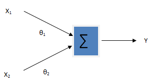
Linear regression is one of the Generalized Linear Model (GLM).  In linear model, the output variable (i.e. dependent variable) is assumed to be a linear combination of input variables (i.e. independent variables). The output variable takes continuous values. Here the input and output variables both are expected to be numeric. The figure below shows the simple representation of a linear regression processor. X₁ and X₂ are input variables and Y is the output variable. The learning goal is to find out the hidden parameters θ(also called weights)

\[ Y = \theta_0 + \theta_1x_1 + \theta_2x_2 \]
Here I will discuss single variable linear regression model. We have only one variable (size of the shoe) and based on this variable we will predicting the prize of the shoe. The first job of building linear regression model is to fit the data into a straight line with minimum error. We will use the least squared error approach for this. The equation of the straight line is given by

\[ h_\theta(x) = \theta_0 + \theta_1x \]
Our job is to find the value of θ₀ and θ₁ that minimizes the prediction error i.e minimizes the function
\[ j = \sum_{i = 1} ^ {m} (h_\theta(x^{(i)}) – y^{(i)})^2 \]
This function is also called as cost function. Here m is the total number of training examples (100 in our example), y is the output variable ( price in our example). There are various approaches by which we can calculate the value of theta that can minimize the cost function. One of the approaches is called Gradient Descent. In this method, we decrease the error gradually by calculating the partial derivative of cost function and subtracting it from initial guess of θ. The initial guess may be [0 0] for θ. The algorithm for gradient descent is given by

Where α is called a learning parameter. It controls how fast the algorithm converges to minimum. If the value of α is large, then it converges fast and if the value of α is small it converges slowly. But remember the large value of α sometime may overshoot the minimum and may fail to converge or even diverge.

import matplotlib.pyplot as plt
import numpy as np
 
def plotData(x,y):
 # plots the value of X and y in graph
 plt.figure()
 plt.plot(x,y,'rx');
 plt.ylabel('Profit in $10,000s');
 plt.xlabel('Population of City in 10,000s');
 #plt.show()
 
 
def computeCost(X,y,theta):
 #computes the cost of linear regression
 m = len(y)
 h = np.dot(X,theta)
 return (0.5/m * (np.dot(np.transpose(h - y),(h - y))))
 
def gradientDescent(X,y,theta, alpha, num_iteration):
 # performs gradient descent to learn theta taking
 # num_iters gradient steps with learning rate alpha
 m = len(y);
 for i in range(1,num_iteration):
  theta = theta - np.dot(np.transpose(X), (np.dot(X, theta) - y)) * alpha / m
 return theta
 
 
print 'Plotting data'
 
from numpy import genfromtxt
data = genfromtxt('data.txt', delimiter=',')
 
X = data[:,0] 
y = data[:,1]
 
plotData(X,y)
 
theta = np.zeros((2,1))
 
print 'Initial theta is ' + str(theta[0]) + ' and ' + str(theta[1])
 
# makes vector 2 dimensional explicitly
X = X.reshape(len(X),1)
y = y.reshape(len(y),1)
 
# adds a column on 1's to the X
X = np.hstack((np.ones((len(X),1)), X))
 
# initial cost for theta
J = computeCost(X,y,theta)
 
print 'The initial cost is ' + str(J)
 
# sets learning rate
alpha = 0.01
 
# sets number of iterations
num_iters = 1500
 
# performs gradient descent to minimize cost function
theta = gradientDescent(X,y,theta, alpha, num_iters)
plt.plot(X[:,1], np.dot(X,theta))
#plt.legend('right')
plt.show()